

Author: Amanbir Behniwal
Mentor: Dr. Gino Del Ferraro
Vincent Massey Secondary School
1. Introduction
Machine Learning jobs are growing to become one of the most in de- mand jobs in the world. In the 1940’s, the idea of machine learning first started to grow; it was something that would emulate human think- ing and learning. Machine Learning has since grown to become a big part of our daily lives. For example, in speech recognition software, the software will map the different tones and nuances when someone speaks and try to match this to a specific person. Another example is a translator, which tries to understand the accents of people speaking a language and then translates it to another language. Many applications that we use today, such as Alexa, Siri, and Google Translate, use these machine learning algorithms. Furthermore, we are trying to integrate machine learning into our vehicles. Cars like the Tesla use unsupervised learning algorithms to self-drive in traffic and detect any danger. The future holds many possibilities due to machine learning.
In theory, we input great amounts of data into machine-learning programs, which using statistics, will categorize or predict outcomes by finding and applying patterns in the data. We can further categorize the different types of algorithms used in Machine Learning to supervised, unsupervised learning and reinforcement learning. Supervised learning consists of regression and classification while unsupervised learning consists of clustering and association.
In this report, we will first discuss important terminology needed to understand the contents of the report. We will then begin to dis- cuss the theory behind some of the machine learning algorithms. The algorithms implemented in this report are all regression algorithms, however, we will also discuss the theory behind other algorithms. Finally, we will see how to implement the code. There are GitHub links provided with the actual code.
2. Terminology
Before we can get started with all the theory, we must develop an understanding of some key terminology that we will use quite often when working with machine learning programs. These are some basic terms that we should be familiar with:
2.1 Features
When we are trying to extrapolate from data using a linear model such as a line of best fit, we want the line to have an equation that best fits the data. In general a line has an equation of h = θ0 + θ1x1 + θ2x2 θnxn. Here we consider x1, x2, , xn1, xnthe features. We will go more in depth about this later on in the report.
2.2 Inputs
When we run a python program, we must somehow store the data so that our program knows what we want it to work with. We then take ’input’ of the data in a convenient way for us to work with it. For example, lets say we had a document that contained a few coordinates. We may want our program to take input of this data where the x- coordinates and y-coordinates are stored separately. The program written to complete this process is called ’taking input’. This process is explained in greater deal in the code.
2.3 Outputs
After our code has calculated what we wanted it to, we want to see this information in an organized manner so that we can study it. We then make our program ’output’ this information. Outputs can consist of words, integers, etc.
2.4 Predicted Values
Let us say that we received input of many coordinates and we wanted our program to calculate the line of best fit. When we are testing different equations to see if they best fit the data, we input the same x-coordinates as the ones in our input data. However, our y-coordinates may not always be the exact same as that of the input data. We thus call our y-coordinates predicted values, since they are what our program predicted the coordinate lies at based on the equation that we came up with.
2.5 Expected Values
The values that we get from the inputted data are our expected values since they are the original values that we are comparing the predicted values to.
3. Supervised Learning
Supervised learning is the most commonly used algorithm in Machine Learning and it is also the simplest to implement. When using super- vised learning, we must train the algorithm by pairing labelled inputs with outputs. The program in this stage is trained to look for patterns that correlate the input to the output. When we have provided the algorithm with a good amount of example pairings, the algorithm will be able to apply this to new inputs it receives. We can further split supervised learning into classification and regression.
3.1 Classification
Classification is a type of supervised learning. In classification, our output will always be a category that the algorithm has mapped the input to. An example of this would be our program receiving input of pictures of animals and then outputting what animal they are (their category). We first have to train the program by inputting many pictures of dogs and cats in their respective categories so that the program will be able to establish patterns between the images of the dogs and the images of the cats. After we have inputted a sufficient number of images, the program will get accurate in determining if an animal is a cat or dog when it receives an input that it has not seen before.
3.2 Regression
Regression is another type of supervised learning. In regression, our output is not a category but rather a value such as money or age. We can take for example the price of houses and the total square footage of the house. Using regression, we identify the function that best fits between these values where we have reduced the amount of error as much as we can. We can then use the equation of this line to predict how much a house with a certain square footage will cost.
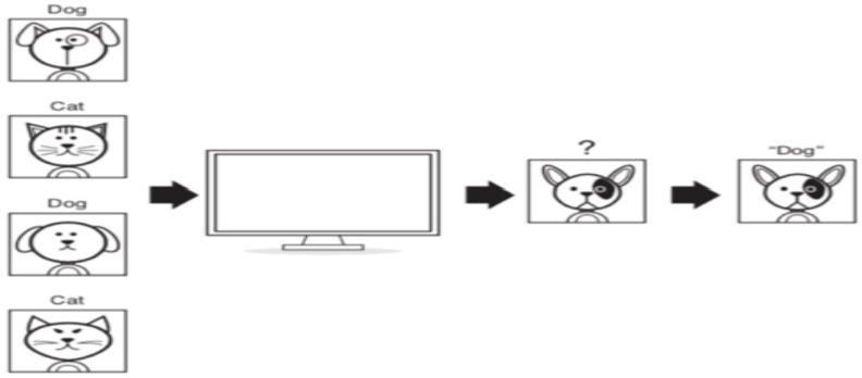
Figure 1: https://medium.com/machine-learning-in-practice/a-gentle-introduction-to-machine-learning-concepts-cfe710910eb
3.2.1 Linear Regression
When performing linear regression, the program will take input of data and plot it on a graph. It will then find a line of best fit and be able to make predictions based on this line of best fit. For example, we can graph the number of hours a student watches TV rather than studying compared to their test scores.
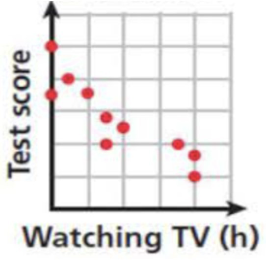
Figure 2: onlinemath4all.com/scatter-plots-and-trend-lines.html
As we can see, the graph looks fairly linear and it only has one feature; the amount of time spent watching TV rather than studying. This makes it a perfect model for linear regression. We want our program to come up with an approximate equation with which we can estimate a students’ test score based on how long they spent watching TV instead of studying. Really, we are looking for our program to find the line of best fit, since this line would be best for extrapolating the data and providing an as accurate as possible estimate of a test score based on the number of hours that were spent watching TV. Our program would then test many different lines until it reaches one line that fits the data better than any other line.
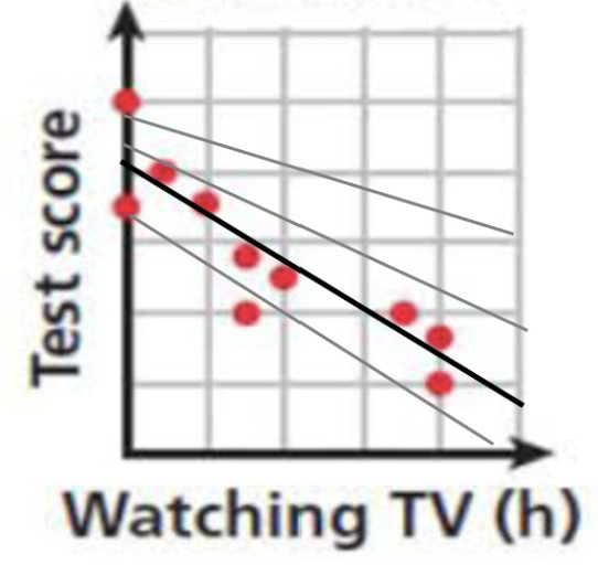
As we can deduce, when calculating the equation of the line of best fit, our slope and y-intercept variables matter a lot. In fact, we are just making changes to these variables to try to find the line of best fit. Machine learning algorithms rely on these parameters (y-intercept, slope/bias, etc.) to run. When we want to find the best model for our data, we need to keep adjusting these parameters so that the direction of our line better fits the data and our predicted values are closer to the expected values. We must then introduce a function that changes these parameters by determining the amount of error that we are getting with the current parameters. This function is called the cost function.
4. Cost Function
The cost function essentially helps our program minimize the error it produces compared to the actual data set. When we are doing linear regression, it is very rare that we will get a data-set where the data fits precisely on a line. Therefore, when we are computing the line of best fit, we want to find a line such that it has the least possible difference (error) between the actual coordinates and the coordinates our line gives (predicted values). There are multiple ways of defining the cost function, some examples are explained further in the following sections.
4.1 Mean Absolute Error
When we take the mean absolute error, we are taking the absolute value of the difference between the predicted y-value and the expected y- value. The reasoning for this is that, since we are adding up all the error for each data point, we want to keep track of how much error we are accumulating.
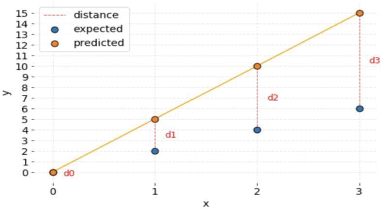
In this graph, the blue points are the original points of the data set, while the orange points are the ‘predicted’ points that our program is currently testing for the line of best fit. As we can see, each direpresents the amount of ‘error’ our model/line produces for each point in the data set.
However, if we add negative numbers (our predicted point is below the original point), our program actually thinks it’s producing less error. To deal with this we take the absolute value, which is always non-negative, so that our program does not add negative error. Then our program can plug this into the formula which is defined as
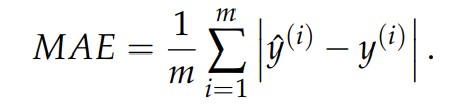
Where mis the number of training examples, yˆ(i) is the predicted value, y(i) is the expected value and i is the index of the data point since we want to sum the error of all the data points.
4.2 Mean Squared Error
When we take the mean squared error, instead of taking the absolute value of the difference between the predicted and expected value, we take their square. In this way, we still don’t add up negative error since any real number squared is non-negative. The equation is defined as:
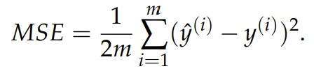
When using mean absolute error, we took the absolute value of the distance between the predicted value and the expected value. We are now taking the square of the area of the square whose side length is the distance between the predicted value and the expected value. All these regions are summed and averaged.
Now that we have discussed how our program will calculate the error that our model/line is producing, we must find a way to minimize the value our cost function is returning. The gradient descent algorithm is one of the most effective ways of doing so.
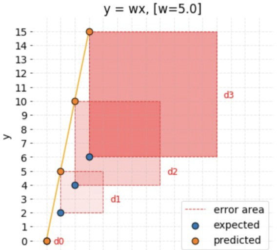
Figure 5: https://gist.github.com/FisherKK/86f400f6d88facbf5375286db7029ca2
For linear regression models, we assume that our data has a linear dependence and therefore can be modelled by using a linear equation as follows;
hθ(x) = θTx= θ0 + θ1x,
where θ0 is our bias (y-intercept) and θ1 is our slope. Then, we want to change our parameters θ0 and θ1 in such a way that our line better fits the data and the cost function produces less error. In batch gradient descent, we update our theta values continuously with the following equation;
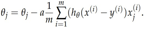
Here, θjis the value that we are updating. Again, mis the size of the data (how many points there are). Alpha here represents the learning rate of our algorithm. If alpha is too big, our program may be a lot faster, but it will not be nearly as accurate in determining the equation of a line of best fit as a smaller value of alpha may be. However, when we use too small a value for alpha, our program will be incredibly slow. It is best to find a good median between these two values.
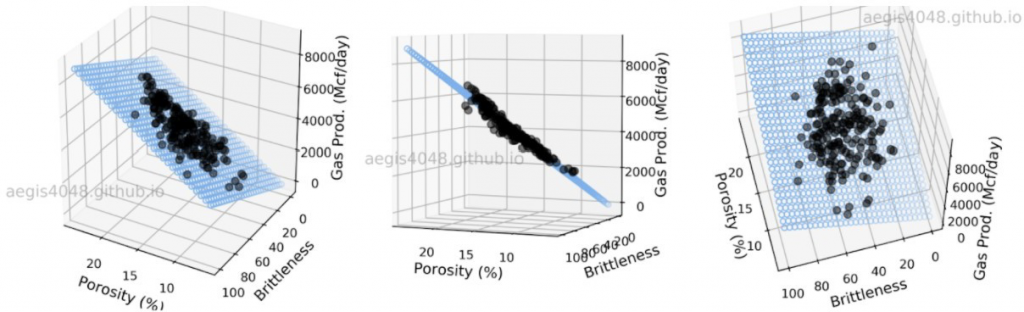
6. Multi-Linear Regression
Now that we have discussed how to optimize our program so that it can calculate the best line of fit with equation h = θ0 + θ1 x1, we think of what we would do when we have multiple features. Currently we have only been working with one feature, which in the example presented, was the number of hours spent watching TV rather than studying. Let’s take another example of the price of a house. When determining the price of a house, we must determine its area, how many rooms it has, how old it is, among other things. In this instance our data when plotted still looks linear however we cannot use the exact same technique as linear regression, since we have more than one feature. We use multi-linear regression in this situation because of its suitability to deal with more than one feature.
Multi-linear regression can be used with as many features as we’d like. Our equation is now
h= θ0 + θ1 ·x1 + θ2 ·x2 + ···+ θn·xn,
where all xirepresent the different features. When we now implement gradient descent, we must use it to update all θiso that our line better fits the data. The cost function can be implemented in much the same way.
The interesting thing to note about multi linear regression is that we need an n-D graph to plot all the points, however, if we take a 3-D graph for example, our program is essentially finding the line of best fit in a plane that best suits all the points.
7. Unsupervised Learning
Unlike supervised learning, in unsupervised learning, we do not train the program with inputs and corresponding outputs. Rather, the pro- gram uses its built-in algorithms to try to find patterns in the unlabelled data and produce an output. For example, if we give input of shapes with different sizes, the algorithm can separate these based on how many sides there are in each shape. In general, unsupervised learning requires much less data then supervised learning. We can further split unsupervised learning into clustering and grouping.
7.1 Clustering
As discussed earlier, in unsupervised learning, we input unlabelled data into our program. Graphing our data, it may look like the following:
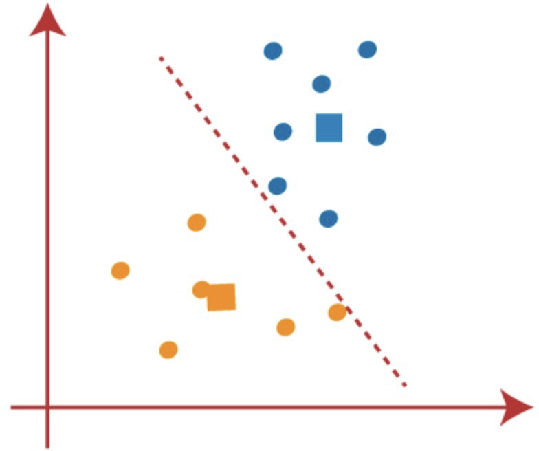
Figure 7: https://www.analyticsvidhya.com/blog/2021/04/k-means-clustering-simplified-in-python/
Once our program has graphed the data, we want our program to try to find patterns in the data. Specifically, clustering algorithms will try to look for clusters of points that seem to be together. The graph could then be divided into the following clusters:
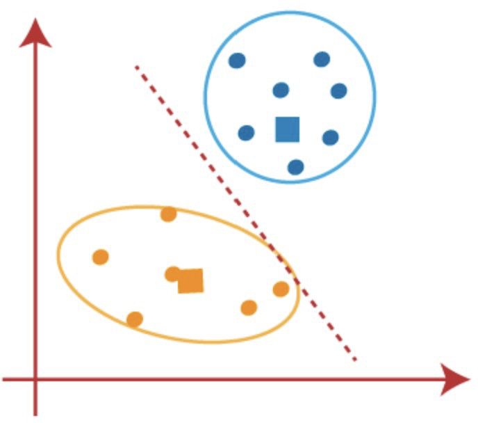
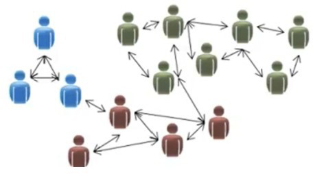
Among the many applications of clustering, we can use the example of social networks. We may want to find which people seem to be very close friends on their social networks so our algorithm would make clusters of people that appear to be close friends.
A more common example in our daily lives would be our spam filter. Our email uses clustering algorithms to try to group spam emails, update emails, advertisement emails, etc. together.
Furthermore, we can classify clustering as hard clustering and soft clustering. In hard clustering, a data point can either belong in a cluster or not. This type of clustering is useful in binary situations such as whether a movie is good or not. On the contrary, when using soft clustering, a data point can belong to many clusters. This is more useful when we may want to determine which books are similar.
7.2 Association
Association algorithms try to see if two items depend on each other. For example, if we take a customer at a supermarket. If this customer has gone to buy bread, then it is very probable that the customer is also looking to buy butter or milk. In this way, we can associate different items based off of their dependency on each other. Many companies use this technique to place associated items away from each other in a store so that the customer see’s many other items on the way and may consider buying additional things. An example of the different associations in a store are given below:
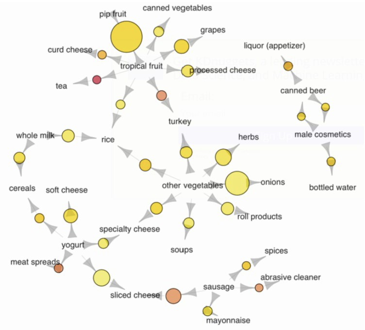
Figure 10: https://annalyzin.files.wordpress.com/2016/04/association-rules-network-graph2.png
8 Reinforcement Learning
In reinforcement learning, the program learns what to do by trial and error in its current environment. We can think of it as the program receiving a reward if it does something correct and a penalty if it does something incorrect. Take the analogy of a child, when a child is young, they do not know what is good or bad. The only way the child can learn is by trying new things. The child may touch something electric, get a shock, then instinctively not go near the thing again. The child now knows that that object is something that shouldn’t be touched because it will hurt. A reinforcement learning program works in a similar way. The difference here is that the machine can try thousands of operations in one second and even though it may start by making very bad decisions, it will learn over time and will become a lot more sophisticated in its decision. We can simulate giving a program a reward or penalty by giving it a score in which, if it does something incorrect, the score will lower, and conversely, if it does something correct, the score will increase. This type of program is based entirely on trial and error on the programs part, it is also one of the closest things to a machine’s own creativity.
One of the most useful implementations of reinforcement learning are simulations. For example, the program can be used to help create the optimal rocket engine for a rocket launch. If we put our in a rocket launch environment in which the environment responds to the actions of our program, we can ‘reward’ the program if it’s helping the rocket launch with its actions or ‘punish’ the program if it’s not helping the rocket launch.
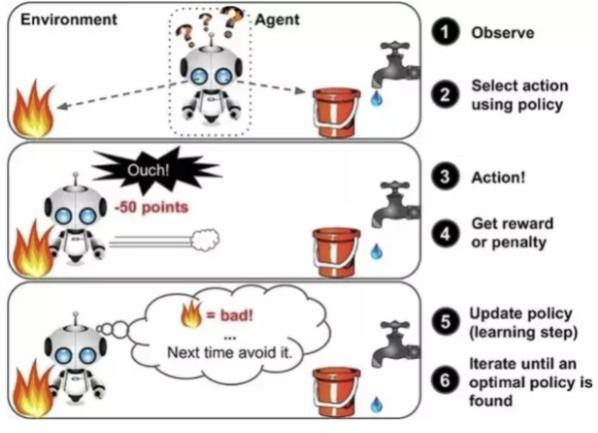
Figure 11: https://riptutorial.com/machine-learning/example/32668/reinforcement-learning
9. Linear Regression Implementation
For the linear regression code, we took input of the population of a city in 10, 000s and its profit in $10, 000. We then plotted all of the coordinates and got the resulting graph:
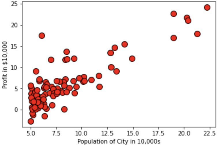
As we can see the graph looks fairly linear, thus we can use linear regression on this.
The full code can be found at: https://github.com/ABehniwal/face-recognition/ blob/main/Numpy-Linear-Regression.ipynb
10. Multi-Linear Regression Implementation
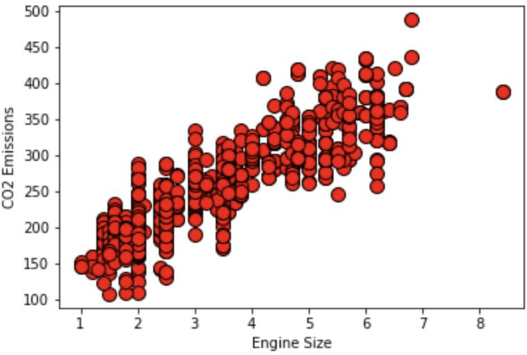
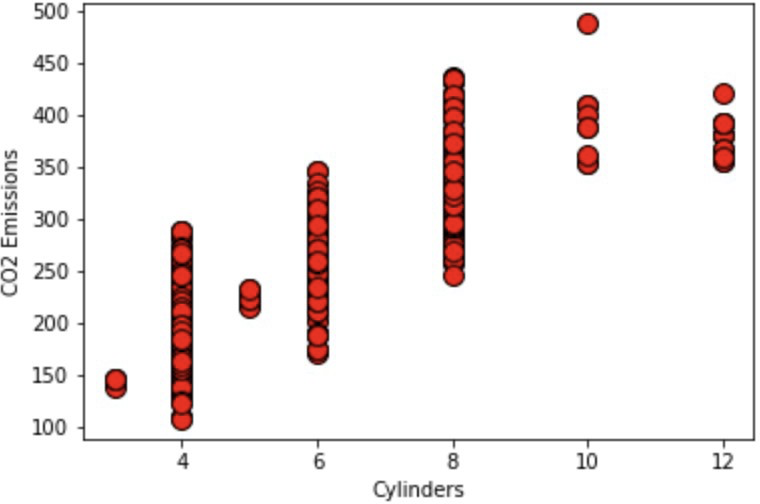
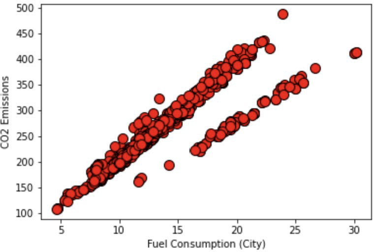
For the multi-linear regression code, we took input of the different features of a car (Engine Size, Cylinders, Fuel Consumption (City), Fuel Consumption (Comb)) and the resulting CO2 emission. We then plotted all of these features of the car separately with the CO2 Emissions to get a visual of how the different graphs look. This resulted in the following graphs.
10.1 Engine Size Graph
10.2 Cylinders Graph
10.3 Fuel Consumption (City) Graph
10.4 Fuel Consumption (Comb) Graph
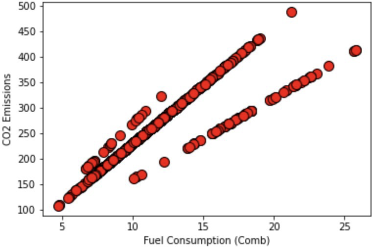
Again, we see that all the graphs look fairly linear, however, since we have multiple different features of the car that we must take into account, we use multi-linear regression. The full code can be found at: https://github.com/ABehniwal/face-recognition/blob/main/Multi-Linear-Regression. ipynb
About the author
Amanbir Behniwal
Amanbir is currently an 11th grader at the Vincent Massey Secondary School in Ontario, Canada. He enjoys challenging myself with difficult math and computer science problems by participating in various contests. Amanbir is an avid fan of Barcelona and has been playing soccer for many years. Amongst other things, he likes to read books, help others with problem-solving, and delve deeper into the field of computer science.