

Author: Mahesh V N
Shanghai American School
November, 2020
What is Machine Learning
Machine Learning is a subset of Artificial Intelligence (AI) which provides machines the ability to learn automatically and improve from experience without being explicitly programmed. Machine Learning is used anywhere from automating mundane tasks to offering intelligent insights. With growing statistics, machine learning gained popularity and the intersection of computer science and statistics gave birth to probabilistic approach in AI. Having large-scale data available, scientists started to build intelligent systems that were able to analyze and learn from large amounts of data. Machine Learning is a type of AI that mimics learning and becomes more accurate over time.
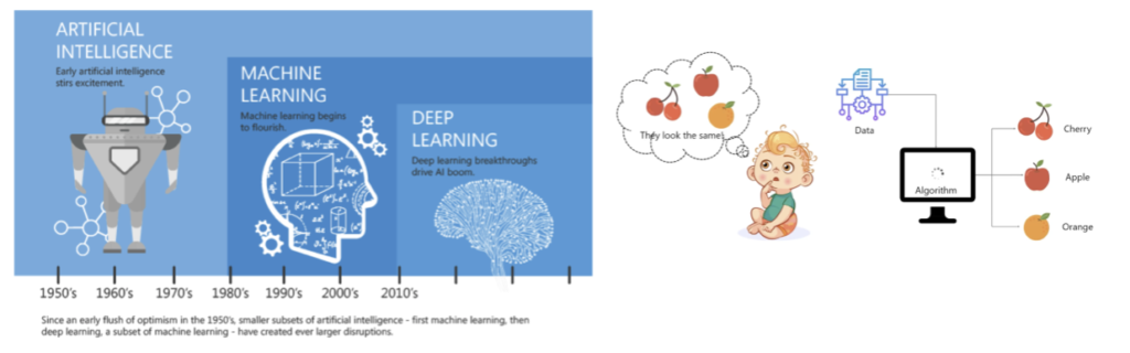
(left) Segmented approach to AI, over the decades (right) Thought process of ML functioning pics. Credit https://towardsdatascience.com/ and www.edureka.com
Applications and Prospects.
Artificial Intelligence (AI) is all around us and we are using it in one way or the other. One of the popular applications of AI is Machine Learning (ML), in which computers, software, and devices learn through data how to make predictions. Companies are using ML to improve business decisions, forecast weather and much more. Machine learning is about training algorithms on a given set of data and make predictions on another set of unseen data. Some of the most common machine learning applications are:
- Learning to predict whether and email is spam or not.
- Clustering Wikipedia entries into different categories.
- Social Media Analysis (Recognise words and understand context behind them) – LionBridge project is a sentiment analysis tool provides users with insights based on social media posts.
- Smart Assistance – analyse voice requests or automate daily tasks as well as adapt to changing user needs – Alexa by Amazon uses all collected data to improve its pattern recognition skills and be able to address user needs.
- News Classification – As the amount of content produced exponentially, business and individuals need tools that classify and sort out the information. With algorithms able to run through millions of articles in many languages and select the ones relevant to user interests and habits.
- Image Recognition
- Video Surveillance – With complex algorithms developed using machine learning for video recognition, at first using human supervision the system will learn to spot human figures, unknown cars and other suspicious objects, soon it will be possible to imagine a video surveillance system that functions without human intervention
- Optimisation of Search engine results – Algorithms can learn from search statistics, they would not be relying on meta tags and keywords, but instead analyse the contents of the page. Suitably this is how – Google Rank Brain works.
Types of Machine Learning approaches
Machine learning is a unique way of programming computers. The underlying algorithm is selected or designed by a human. However, the algorithms learn from data, rather than direct human intervention. The parameters of a mathematical model are learnt by the algorithms in order to making predictions. Humans don’t know or set those parameters — the machine does.
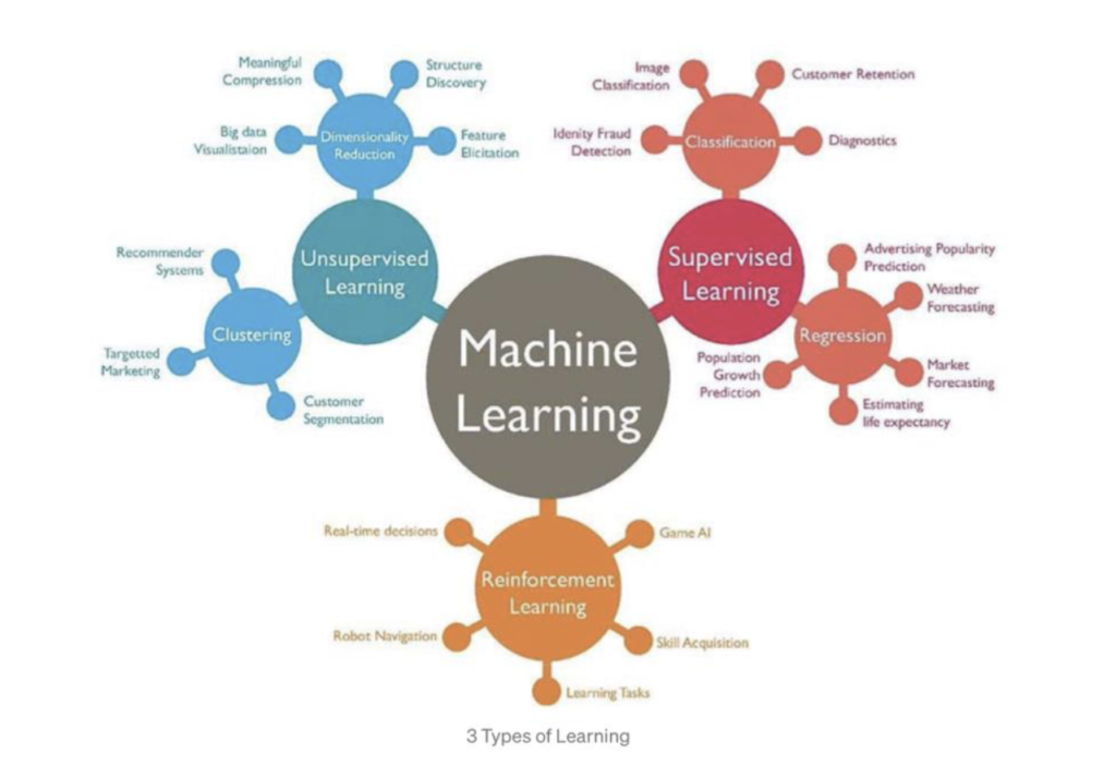
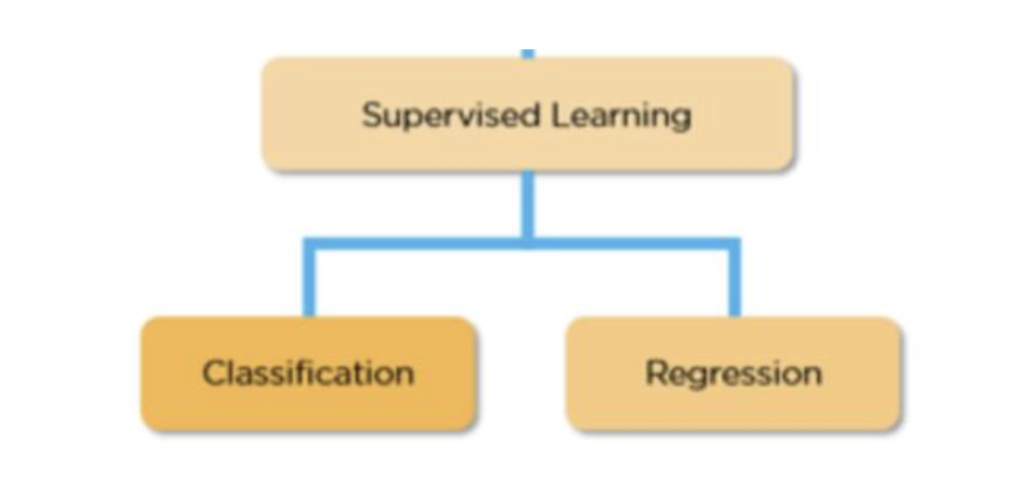
To explain in simple terms Machine Learning is using a data set to train a mathematical model which is fed with enough sample to have a predictable analysis and output a sensible result. Machine Learning can be divided into a series of subclasses: Supervised Learning, Unsupervised Learning, and Reinforcement learning. The supervised learning category is further divided into Regression and Classification for more streamlined approach to a task, which results in faster and accurate results.
Nomenclature of Machine Learning terms: A feature is an individual measurableproperty of the phenomenon being observed, e.g. square footage of a house to predict the house’s cost, 2D image input to perform object recognition, etc… It is a characteristic of the data that is used as input of the ML algorithm and for this reason it is often used as a synonymous of the ML input and it is commonly denoted as x.
The output of the algorithm is also called “prediction” or “outcome” and it is denoted with “y hat”. The label of the machine learning algorithm is usually denoted with y. So, for instance, the purpose of a supervised algorithm is to use input x to generate the output “y hat” which is as close as possible to the real outcome y.
Supervised Learning
Supervised learning is an approach to creating artificial intelligence (AI), where the program is given labeled input data and the expected output results. The AI system is specifically told what to look for, thus the model is trained until it can detect the underlying patterns and relationships, enabling it to yield good results when presented with never-before-seen data. Supervised learning problems can be of two types: classification and regression problems. Examples are: determining what category a news article belongs to or predicting the volume of sales for a given future date.
How does supervised learning work?
Like all machine learning algorithms, supervised learning is based on training. The system is fed with massive amounts of data during its training phase, which instruct the system what output should be obtained from each specific input value.
The trained model is then presented with test data to verify the result of the training and measure the accuracy.
Types of Supervised learning
Supervised learning can be further classified into two different machine learning categories:
- Classification
- Regression
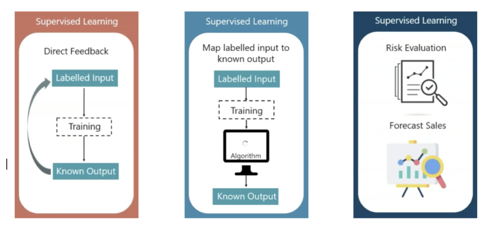
In case of supervised learning shown in Fig (3.1 – a) we train the algorithm to take up data and come up with an output which is known as this model is fed with input which is labelled. In the (fig – 3.1(b)) The sample Maps the labelled input into a known output. Few of the application of the supervised learning is risk evaluation and forecast of sales in a given business.
Classification in Machine Learning.
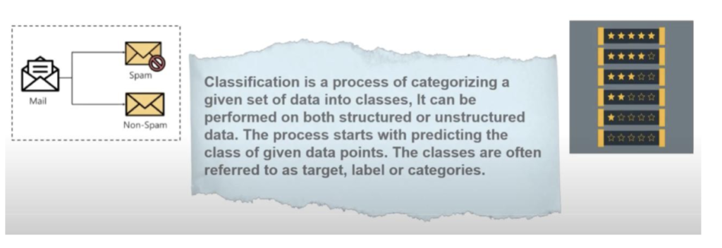
Classification is a supervised Machine learning approach used to categorise a set of data into classes. Typically our outcomes are CLASSES or categories. For example, this is a case where a user is trying to predict what is in a given image. Wherein a clear demarcation is provided.
Classification to start with has two sub categories basically named as Lazy Learners and Eager Learners. In case of the former it just stores the training data and wait until a testing data is presented, although they have more time predicting data. Whereas in the later case, they construct a classification model based on the given training data before performing the task of predictions, they consume a lot of time in training and less time in prediction as they commit to a single hypothesis that shall work for the entire space.
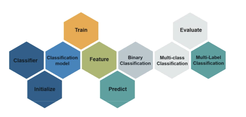
In the Figure – 4.0 (above) we have a classifier, which in most cases is an algorithm used to map an input data to a specific category. Classification model is trained to predict the class or category of the data.
Classification problems can be divided into two different types: binary classification and multi-class classification.
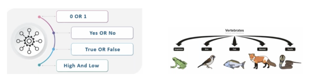
Binary classification has two outcomes based on the categories specified for therequired output (Example: the output is to be noted only as a dog or a cat.) .
In case of a multi-class classification the outputs or predictions are more than two (in general a group of M possible predictions). The goal of the algorithm is to predict the specific output among the possible M.
Note: Classification is going to be discussed further in more detail in further sections.
Regression Machine Learning
Regression is a predictive statistical process where the model attempts to find the important relationship between dependent and independent variables. The goal of a regression algorithm is to predict a continuous number such as sales, income, test scores and so on. Before attempting to fit a linear model to observed data, a modeler should first determine whether or not there is a relationship between the variables of interest. This does not necessarily imply that one variable causes the other (for example, higher SAT scores do not cause higher college grades), but that there is some significant association between the two variables
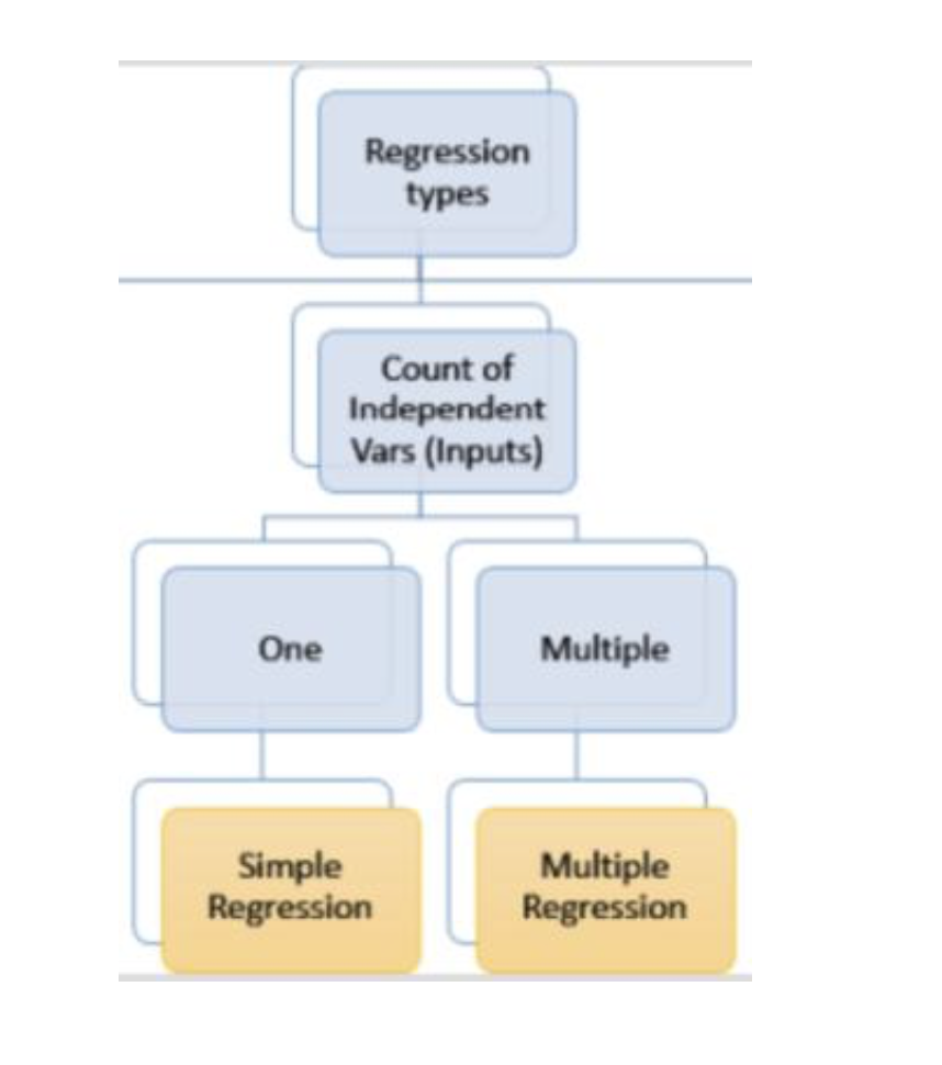
Types of Regression: Simple (Univariate)
Conditions: One variable is considered
A Mathematical Approach into Linear Regression
Y = ß0 + ß1 X, is theform of equation of linear regression. Where X isthe independent variable, and Y is the dependent variable. ß0 is the slope of the line and beta1 is the intercept ( the value of y when x = 0 ). Fitting this equation into linear regression model of the data provides successful results in prediction of the unknown data. The fitting procedure consists in finding the parameter ß0 and ß1 that best fit the data. In machine learning terms, this means to “learn” the parameters a and b that produce the least error in fitting the data.
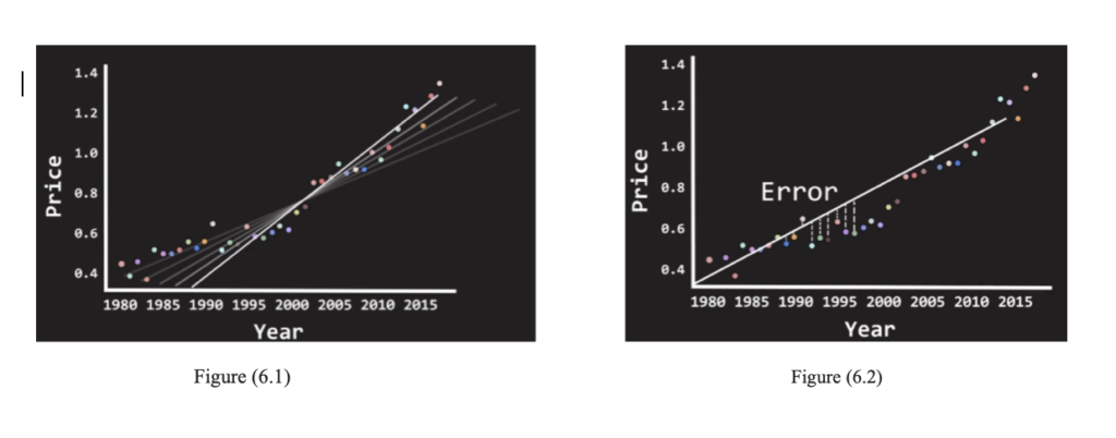
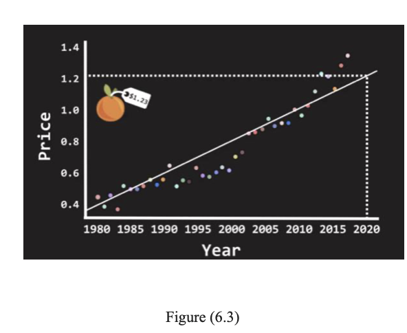
Least-Squares Regression
This is the most common method for fitting a regression line into the Regression model. It is the process of calculating the best-fitting line for the observed data by minimizing the sum of the squares of the vertical deviations from each point to the line (vertical deviation being 0 for the point fitted line). The deviations are squared and summed in order to prevent the cancellation between negative and positive values. Least-Square Regression uses the “Ordinary Least Square” or “OLS” method to determine the best fitting line. This is the method where a line is chosen that “minimizes the distance between every point and the regression line”. In figure 6 we give a visual description of this process. The distance is also known as the error in the system (see Figure(6.2)). In Figure 6.1, as an example, we consider the price of the commodity and the year of the production.
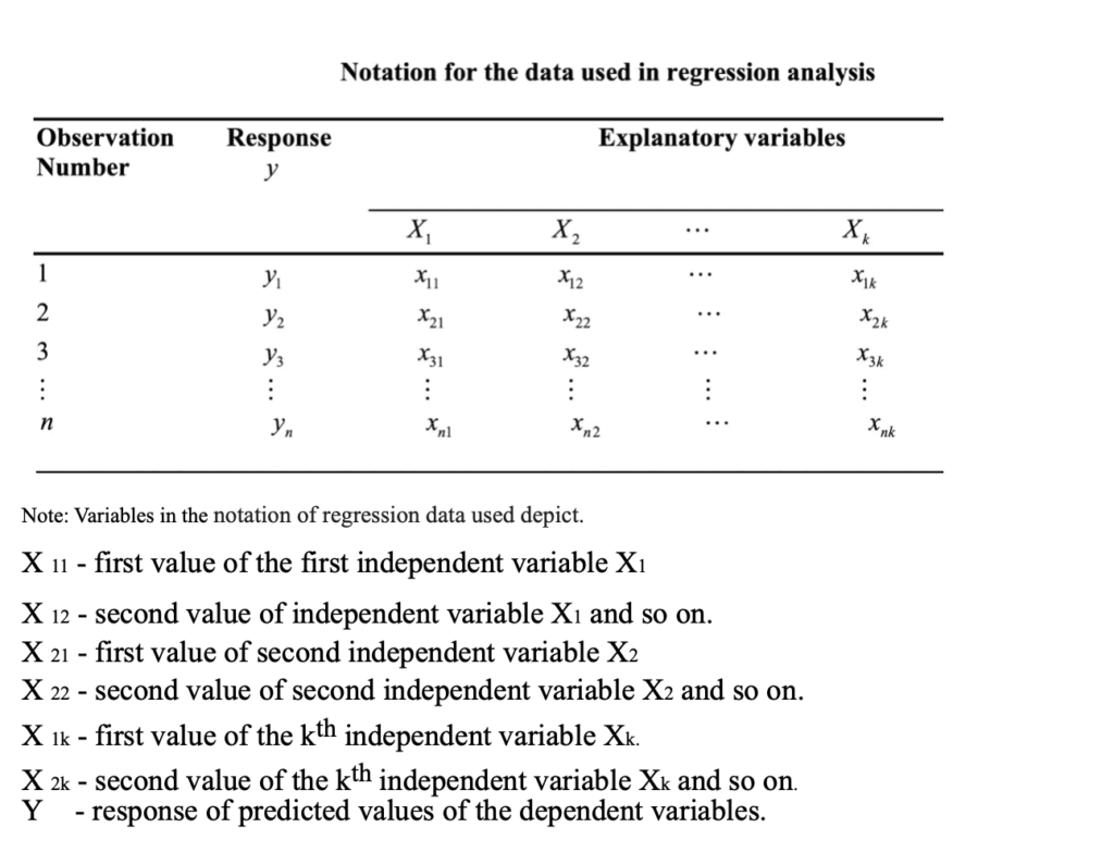
Once the best fitting line has been found, we can use it to predict the price of the commodity in the year 2020 based on all the data from the previous years.
What is Multiple Linear Regression?
Multiple linear regression is the most common form of linear regression analysis. As a predictive analysis, the multiple linear regression is used to explain the relationship between one continuous dependent variable and two or more independent variables. The independent variables can be continuous or categorical.
A Mathematical approach
Multiple linear regression attempts to model the relationship between two or more explanatory variables and a response variable by fitting a linear equation to observed data.
Model for Multiple Linear Regression, given n observations,
y = ß0 + ß1X1 + ….. + Xnßn + e
Where the values depict,
y – predicted value of the dependent variables.
ß0 – the y-intercept calculated when the other values are set to 0.
ß1X1 – regression coefficient (ß1) of the first independent variable (X1), which depicts the change in the predicted y – value with change in the independent variable.
ßnXn – regression coefficient of the nth independent variable (feature).
e – variation in the prediction of y value, also known as the model error.
(X1, X2, X3, …. Xn ) are the dependent variables factoring into the y value.
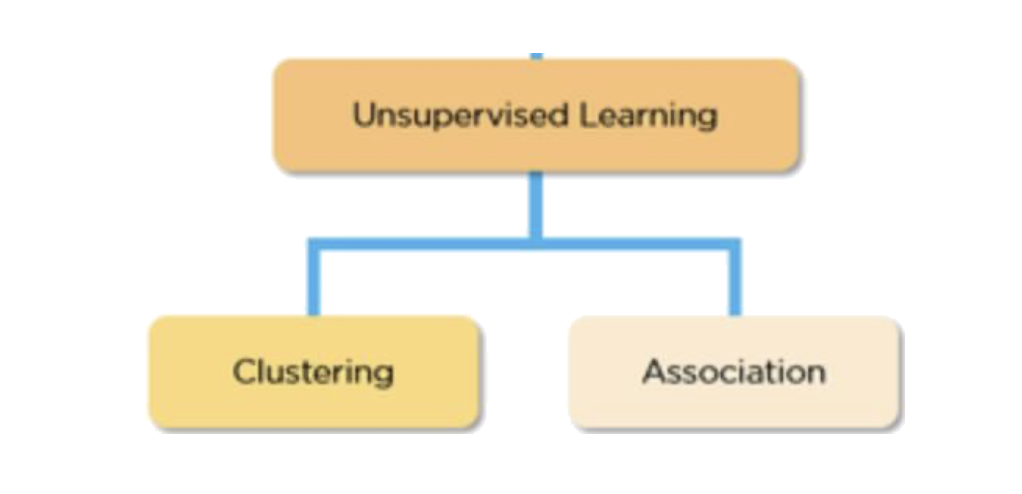
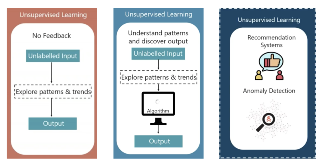
Unsupervised Learning
Unsupervised Learning is often used in the more advanced applications of artificial intelligence. It involves giving unlabeled training data to an algorithm and asking it to pick up whatever associations it can on its own. Unsupervised learning is popular in applications of clustering (the act of uncovering groups within data) and association (predicting rules that describe data).
In the Figure – 4.0 (above) we have a classifier, which in most cases is an Algorithm which is used to map an input data to a specific category. Classification model predicts/draw conclusion of the class or category the data needs to be segregated. A feature is an individual measurable property of the phenomenon being observed. Binary classification has two outcomes based on the categories specified for the required output (Example: the output is to be noted only as a dog or a cat.) . Whereas in multi-class classification in each sample is assigned to a set of labels or targets (more than two).
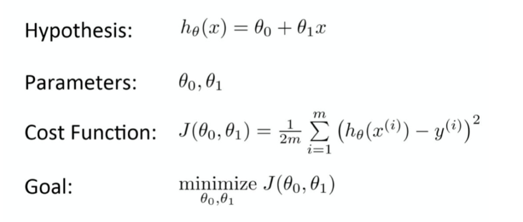
Cost Function and Gradient Descent
A measure of how wrong the model is in terms of its ability to estimate the relationship between x and y is a cost function of the Machine Learning model (in the examples above OLS is a cost function for linear regression). Which is typically expressed as a difference or distance between the predicted value and the actual value. The Objective of a Machine Learning model is find parameters, structure etc that minimizes the cost function.
The best-fit line is found by minimizing the difference between the actual value and the predicted values. Linear Regression does not apply brute force to achieve this, instead it applies an elegant measure known as Gradient Descent to minimize the cost function and identifies the best-fit line.
Gradient Descent is an iterative optimisation algorithm for finding the local minimum of a function. The process of determining the local function is by taking steps proportional to the negative of the gradient of the function at the current point. Gradient descent is defined by the algorithm defined as
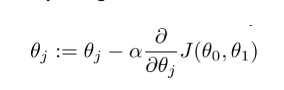
The goal of the gradient descent algorithm is to minimize the given cost function by performing two steps iteratively.
- Compute the gradient (slope), the first order derivative of the function at that point.
- Make a step (move) in the direction opposite to the gradient, opposite direction of slope increase from the current point by alpha times the gradient at that point.
Alpha is the learning rate – a tuning parameter in the optimization process, which determines the length of the steps to be taken.
Make a step (move) in the direction opposite to the gradient, opposite direction of slope increase from the current point by alpha times the gradient at that point.
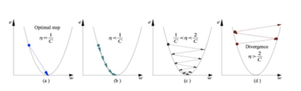
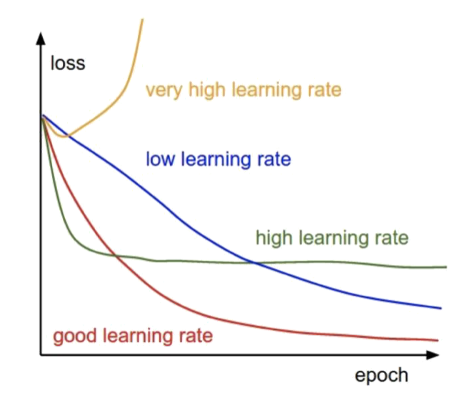
We are going to examine different methods of determining the steps with Alpha – the learning rate
a) Learning rate is optimal, model converges to the minimum.
b) Learning rate is too small, it takes more time but converges to the minimum.
c) Learning rate is higher than the optimal value, it overshoots but converges ( 1/C < η <2/C).
d) Learning rate is very large, it overshoots and diverges, moves away from the minima, performance decreases on learning.
Classification: Logistic Regression
Logistic regression is a supervised learning classification algorithm used to predict the probability of a target variable when the target has only two possible outcomes, for instance either 1 (stands for success/yes) or 0 (stands for failure/no). Logistic Regression is further classified into to categories namely binomial and multinomial.
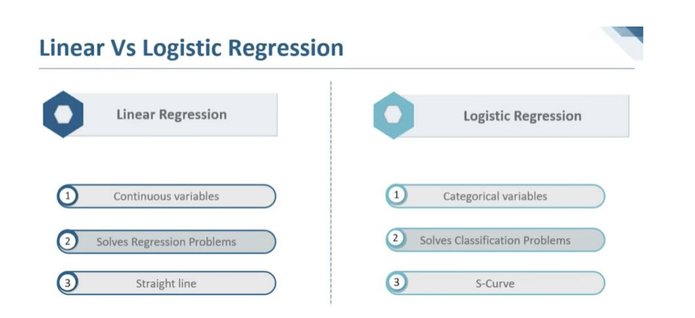
Linear Regression vs Logistic Regression
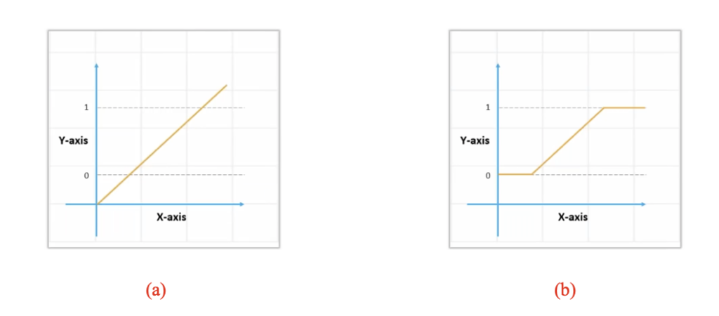
In the above shown figure 7.1 (a), the value of Y or the dependent variable lies within a range that can take values beyond 0 and 1. Whereas in the case Logistic Regression (figure 7.1(b)) the outcome/predictions will be between 0 and 1 (see figure 7.1(b) and figure 7.2). To have then a binary output, we threshold every value below 0.5 to 0 and every value above 0.5 to 1 (see figure 7.2).
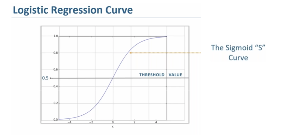
Sigmoid Function Curve
The sigmoid function curve also known as the S-curve is used in conversion of any values between negative infinity to positive infinity to a discrete values or in our into binary format of 0 or 1 (refer figure 7.2). The S-curve has values of x-axis between -4 to +4 (in our example) is considered as the transition values. Considering the data point value as 0.8 which falls neither in the category of a discrete 0 or a discrete 1. The concept of “Threshold Value” 0.5 is applied to get a discrete value of 0 or 1. The process is of threshold value application is dependent on the value of given datapoint is greater or lesser than the threshold value. If the datapoint is greater than threshold the discrete predicted value is 1 or the discrete predicted datapoint is 0 otherwise.
Practical Use – Linear vs Logistic Regression.
Let us consider Weather forecast of a particular given calendar day. Logistic regression is used in predicting the outcome of the weather for a possibility of a rain, snow, tide or a sunny weather. The above predictions of a possibility fall in to the category of Yes or No which are discrete outcomes. If we consider further, Linear Regression can also be applied to weather forecast such as the temperature of a given day (same calendar day, considered earlier) . Since the temperature of day is a continuous value, linear regression can be applied to the same set of samples to predict the outcomes.
Linear Regression – coding exercise
To develop practical coding skills I have implemented Linear Regression in python from scratch. The problem that I consider was to predict the price of a house from its square footage, using existing real data. The code notebook can be found here: https://github.com/gdelfe/Machine-Learning-basics-course/blob/master/Exercise1/exercise1_MLbasics.ipynb
About the author
Mahesh V N
Mahesh is a student at the R. N. Shetty Institute of Technology in Bangalore.