Analysis of the Duration of California Real Estate on the Market

---

Abstract

In investment, timing of buying and selling is crucial to profits. In the real estate community, there is often debate amongst investors on the perfect timing to sell real estate. While many contend that the perfect timing is during the summer or spring, there has been little statistical support of these theories. The purpose of this paper is to locate the optimal time for real estate sales in California based on length of time on the market. In this paper, multiple graph types are used in order to determine a concrete pattern that can be used as a basis for future real estate sales. Cyclical functions are used for the majority of the paper as they are a commonly used as a tool to analyze monthly variances. These functions are based on a twelve month scale and vary in percent change of average days of California property on the market. This way, the analysis can emphasize more on the individual changes from month to month rather than year to year. This means that the data compiled across multiple years is analyzed at the same time for each month. To analyze this data, a mean, median, or even a LOESS curve can be utilized to find the trend of the average length real estate is on the market. The mean refers to the value of all variables divided by the number of variables, whereas the median refers to the value that separates the upper half of the data from the lower half. In a LOESS curve, the points are sectioned off into different groups. Within these groups, points are calculated using a focal point, and are determined based on the points closest to the focal point. The closer the point to the focal point, the larger the weight. This is done for every point in the model until the LOESS curve is complete. This can make the model less influenced by one or more outliers. Through the use of these methods, the optimal time for selling real estate based on average days on the market can be found.

Overall Changes:

To look at the optimal sale time in California, aggregated real estate data was pulled from Zillow ranging all the way from January of 2010 to December of 2019 (“California Home Prices”). As can be seen through the following charts, the average days of real estate on the California market has seemed to drop over the course of ten years from almost 100 days on the market to slightly above 50.

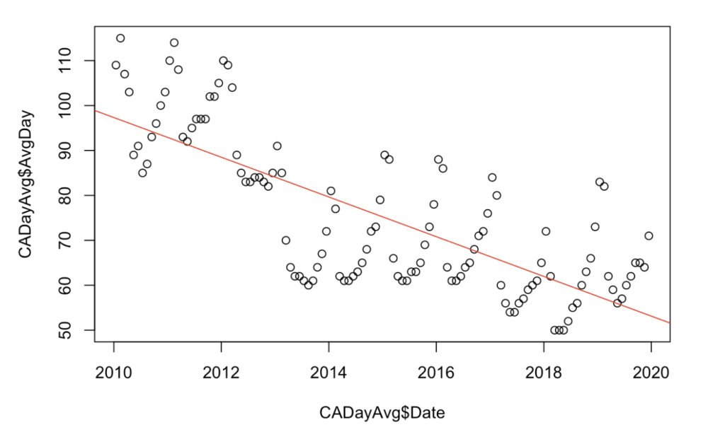
This change could have been caused by a variety of factors, including the Great Recession from the end of 2007 until 2009. While the data only tracks the changes starting from 2010, the effects are still great enough to be seen. The Great Recession was caused by the housing market booming then busting when financial institutions over-lended and over-marketed mortgage backed securities at exorbitant levels to sometimes unqualified borrowers (Hall). After the recession, consumers were then hesitant to invest in the very market that had caused the crash. The high levels of days in which real estate was on the market demonstrates the tentative investors. However, as can be seen from 2012 onwards, the days on the market fell as people slowly gained confidence in real estate, with the days on the market generally stabilizing from 2013 to 2017, followed by an even further decrease.

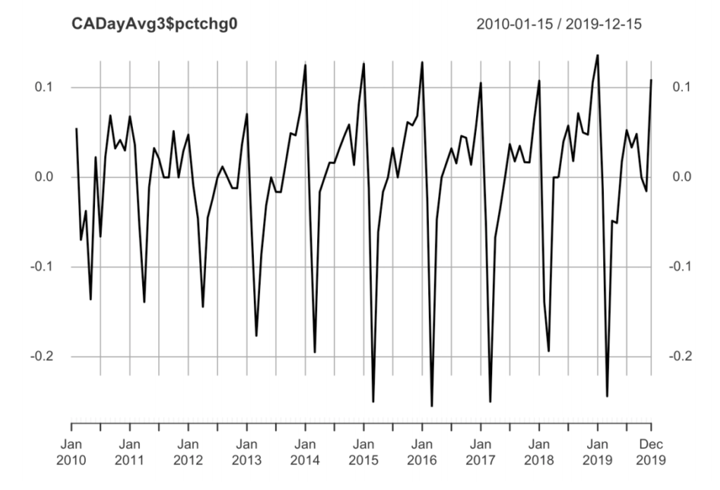
When looking at initial data displayed in Figure 1, one can almost instantly recognize the cyclical form taking place from 2013 to the end of 2019. This initial instinct led to the creation of a graph depicting the percent change from one month to the next over the course of these ten years. From this chart, my initial theory was confirmed and it can be seen that the average days on market of real estate indeed has a cyclical pattern.

Monthly Basis:

After the assurance of a repetitive, reliable pattern from year to year, the next step was finding a way to demonstrate the differences in monthly averages of length of California real estate on the market. To do this, the x-axis was set to a month by month basis (Figure 3). Each year is represented by a scale of colors, with the oldest data from 2010 being the darker blue, and the most recent from 2019 being lighter blue. This way, the data would emphasize each month and the differences between those months.

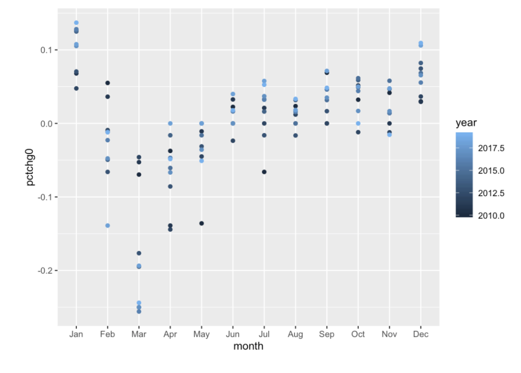
There were no significant outliers from year to year. For example, the darkest blue colors did not show that the percent change in days on the market to stay the same from January to February, rather, for almost all years, as can be seen through the tight clusters, there seemed to be specific months where the percent change would be similar, whether it be 2010 or 2019. The month of December demonstrates this. From 2010 to 2019, the month of December has stayed between zero to a little above 0.1 percent change in average days of real estate on the California market.

The data points were usually in close clusters, which caused the mean and median to be relatively similar and consistent throughout the twelve months. In Figure 4, the red line represents the median percent change of each month in average days on the market for California real estate while the blue represents the mean of the percent change of each month. The average standard deviation of the points from each month is 0.0375. Some months varied more than others; months such as March had relatively larger standard deviations of 0.083, while months like June had smaller deviations of only 0.015. Overall, the standard deviation is still quite minimal. The green line depicted below demonstrates the mean of the percent change from year to year, which is-0.00034%. When the mean and median (red and blue) are so closely related, it can be said that the data has minimal outliers and that both the mean and median are accurate measures of this set of data points.

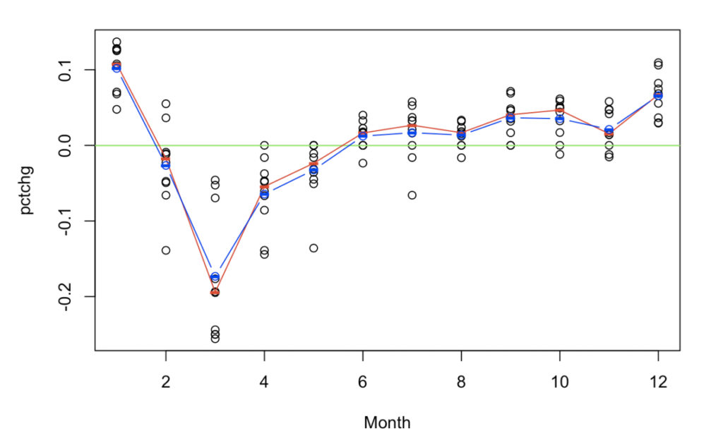
Both the mean and median in Figure 4 display the lowest point to be in March, followed by a sharp increase in April and a more gradual incline through to January, where it once again drops dramatically. This has high implications in that it could potentially mean that the month with the shortest days on the market for real estate is March. The high increase from November to January is likely due to low demand during holiday season as most are busy with familial obligations (Fuscaldo). On the other hand, the dip in April and March is most likely caused by the high demand as families start to search for a home before the school year begins (Thorsby).

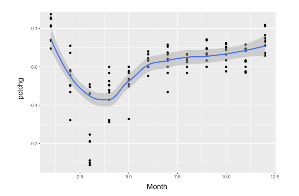
Figure 5 denotes a similar chart to Figure 3 and 4, except instead of a mean or median, it uses a LOESS residuals curve to find the curve for average days on the market for Californian real estate. In Figure 5, the blue line demonstrates the LOESS curve which is based on the weight of local points, while the gray area following the blue line represents the confidence band. The confidence band is the uncertainty in a curve based on limited data. As can be seen in the chart below, the confidence band is fairly thin, meaning that the difference between the highest and lowest points are significant.

As can be seen in Figure 5, the LOESS curve conveys similar, but not exactly the same information. It still shows that November through January have the longest durations for average days on the market, as well as significant drop in the spring. However, recall that in Figure 4 both the mean and medians displayed March to be the lowest point, but according to the LOESS model it seems that April is the lowest point. The real life theory is still supportive of why consumers have higher demand for housing, yet what is causing the numerical differences? This all leads back to the way LOESS curves are constructed. A LOESS model can be more accurate than the mean or median because it is more influenced by the local points near the focal point, whereas the mean and median can shift quite easily due to a couple of low values, such as in Figure 3 where March is quite low compared to Figure 4. As mentioned earlier, March’s standard deviation is larger compared to the other months, which could be the reason the LOESS curve was only different from the mean and median in this month and not the others.

Conclusion:

Although there are a few minor differences between the median/mean and the LOESS model, the general shape of the curve still suggests that the lowest point is in the spring from March to April. This means that the lowest average days California real estate is on the market is during those months. The decrease could be caused by a rise in demand due to increased pressure to purchase in anticipation of a new job after the summer or new school. The worst time for real estate sales in regard to length of time on market is typically in the winter, where families and individuals are busier with the holidays and are more reluctant to see open houses.

Mentor: Dr. Peter Kempthorne, Massachusetts Institute of Technology

---