

Author: Roshna Shaik
Osmania University.
November, 2020
Abstract
Pharmaceutical Preparation Manufacturing U.S. industry comprises establishments primarily engaged in manufacturing in-vivo diagnostic substances and pharmaceutical preparations (except biological) intended for internal and external consumption in dose forms, such as ampoules, tablets, capsules, vials, ointments, powders, solutions, and suspensions.
The Producer Price Index (PPI) measures the change over time in the prices received by domestic producers of goods and services. More detailed indexes are used as sources for industry analysis and contract escalation in the public and private sectors.
PPI data are critical inputs into the development of sensitive economic indicators, including estimates of gross domestic product and industrial productivity.
Pharmaceutical companies have deep scientific knowledge gained from decades of experience with several viruses. Companies are researching vaccine candidates and undertaking inventories of research portfolio libraries to identify additional potential treatments for R&D to combat COVID-19.
Some are exploring ways to use existing technologies that provide the ability to rapidly upscale production once a potential vaccine candidate is identified.
So, it becomes crucial to estimate the value of Producer Price Index of Pharmaceutical Industry: Preparation and Manufacturing in this pandemic.
1. Introduction
1.1 Producer Price Index
The Producer Price Index (PPI) program measures the average change over time in the selling prices received by domestic producers for their output. The prices included in the PPI are from the first commercial transaction for many products and some services.
The data of Producer Price Index of Pharmaceutical preparation and manufacturing industry is obtained from ‘FRED’. The obtained data has monthly frequency starting from June 1981. This particular data has been utilized for our project.
1.2 Analysing Full Series
The plot for the full series shows that there is a significant increase in producer price index in March 1998 from the previous month.
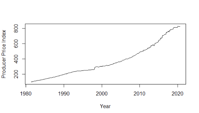
The plot shows increasing trend overall indicating a non-stationary trend. We have used “ndiffs” function of “forecast” library to estimate the number of differences required to make the time series stationary. The result was 2.
1.3 Second Order Differencing
In March 1998, the Food and Drug Administration (FDA) approved usage of few drugs resulting in significant increase of Producer price index from 265.0 to 291.0
This led the ndiffs function to estimate the second order of differencing to make the series stationary.
Later, we broke the entire timeline into two parts to exclude March 1998 period.
- First 10 years
- Last 10 years.
Then, the ndiffs function indicated first order of differencing for both the time periods.
2. First 10 Years
2.1 Auto Regressive Models
The data of first 10 years is converted to first order difference log data. We look for the best Auto Regressive model plotting the Akaike Information Criterion (AIC) for values up to 17.
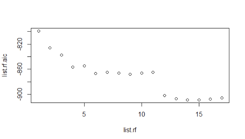
We see that AR model 14 has lower AIC value. Increasing the autoregressive order from 10 improves the fit here. To keep the model consistent with constraints of what models can be fitted, we had to limit the autoregressive order to 12 and fitting the MA terms.
2.2 Moving Average Models
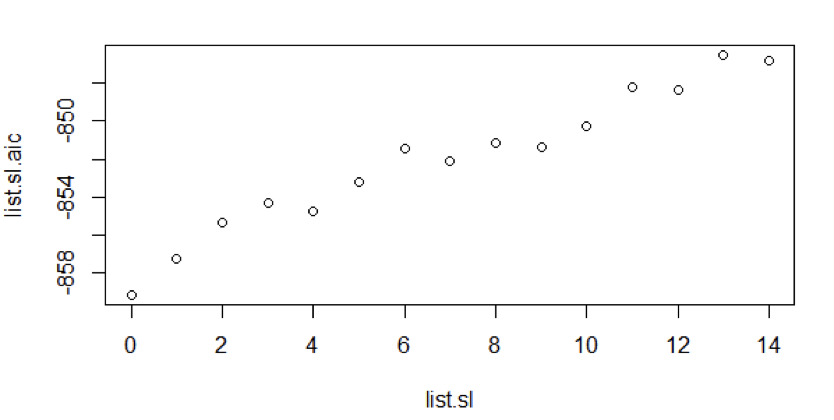
Using the ARIMA function, we’ve plotted AIC values keeping the AR model value 12 i.e., constant and Moving Average values variable up to 14.
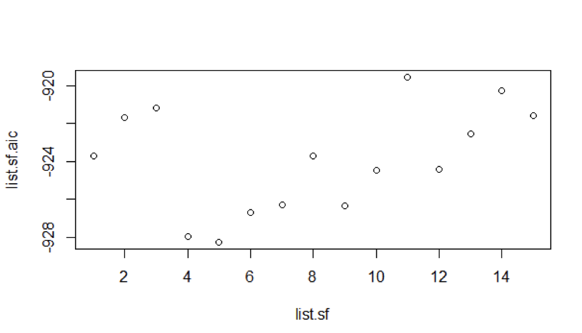
From the figure 3, we can see that for Auto Regressive model 12, Moving Average model 5 suits the best.
2.3 ARIMA Models
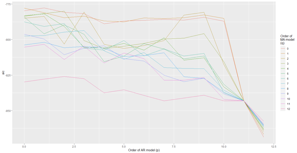
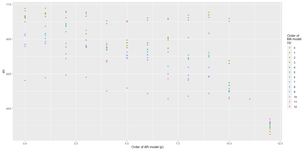
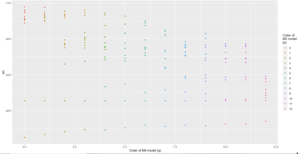
We have plotted AIC values of about 130 models with order of the autoregressive model varying from 0 to 12, the order of the moving-average model varying from 0 to 9 and degree of differencing equal to 1.
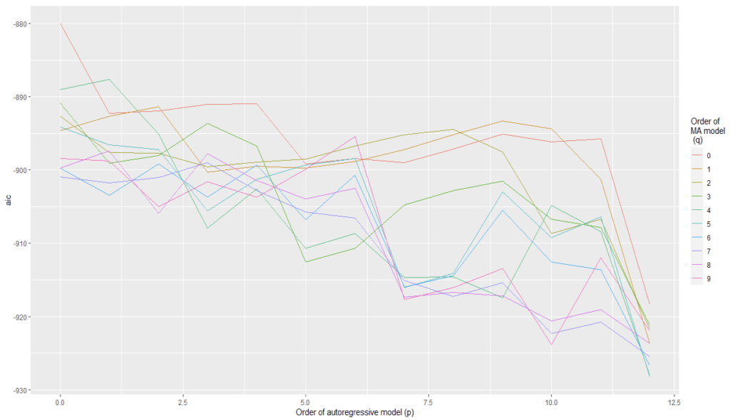
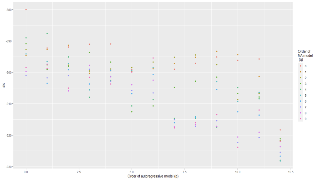
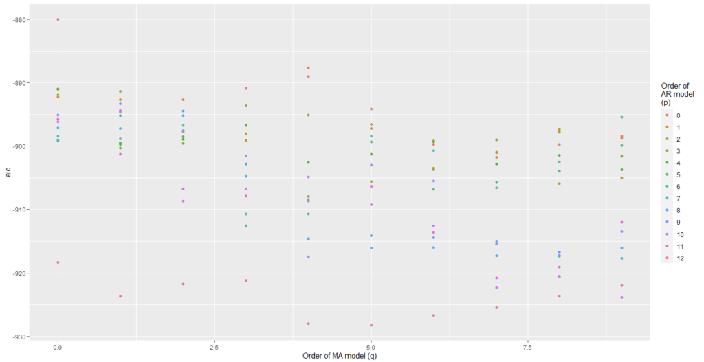
From Figure 5 and Figure 6, we can conclude that for Auto regression model 12 and moving average model 5 are the best one.
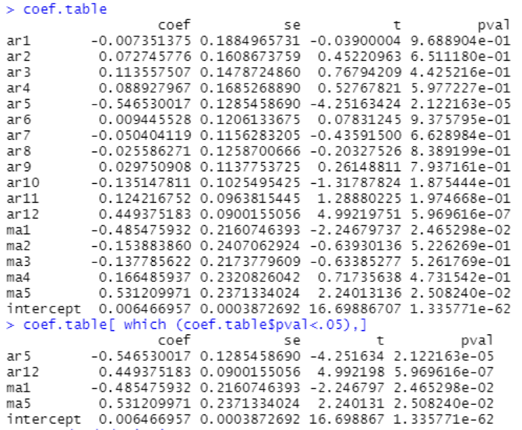
The coefficients table xx and the previous observations suggest that there tends to be a 5 month reversal effect but annual changes year over year tend to repeat themselves. There might be 5 months reversal that is consistent with managing expectations of the stock holder of the companies.
3. Last 10 Years
3.1 Auto Regressive Models
The data of last 10 years is converted to first order difference log data. We look for the best Auto Regressive model plotting of the Akaike Information Criterion (AIC) for values up to 14.
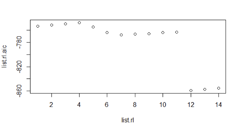
Figure 7: AIC values of AR model for last 10 years data
We see that AR model 12 is the best due to its lower AIC value.
3.2 Moving Average Model
Using the ARIMA function, we’ve plotted AIC values keeping the AR model value 12 i.e., constant and Moving Average values variable up to 14.
From the figure 7, we can see that for Auto Regressive model 12, the Moving Average model 0 suits the best. So we have no MA terms.
3.3 ARIMA Models
We have plotted AIC values of about 168 models with order of the autoregressive model varying from 0 to 12, the order of the moving-average model varying from 0 to 12 and degree of differencing equal to 1.
From Figure 8 and Figure 9, we can conclude that Auto regression model 12 and moving average model 0 are the best one.
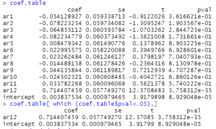
With no Moving average terms, the producer price index is less affected by recent variations in producer price index. The past errors of the prediction model are not predictive of future production levels. So, the fact that past prediction errors are not very helpful suggests that the production process is perhaps stationary with a shorter memory.
4. Comparing Parameters of Two Models
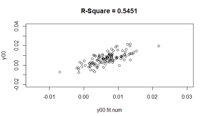
4.1 R-Square
From figure 6, For the ARMA model (12,1,5) of first 10 years, the r-square value is equal to 0.5451
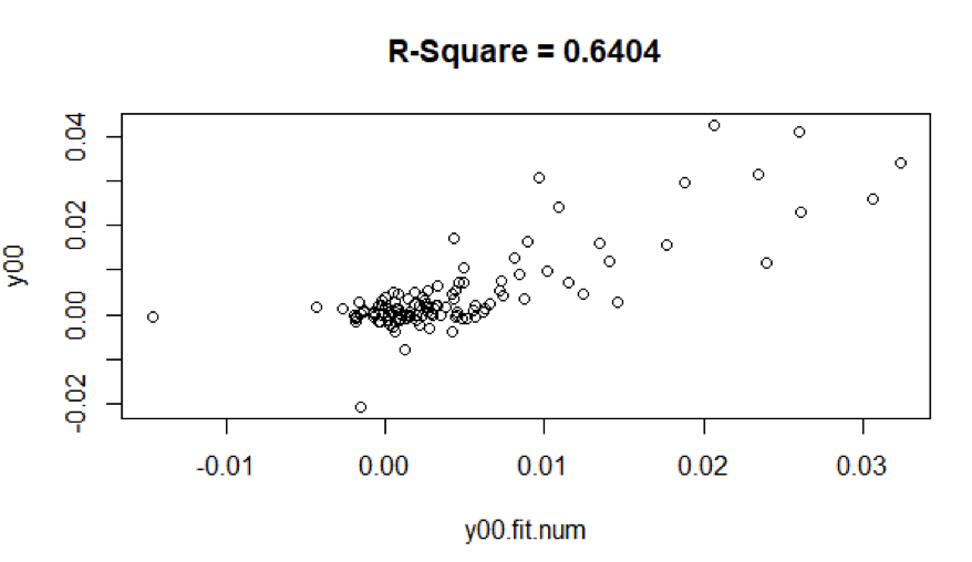
From figure 7, For the ARMA model (12,1,0) of last 10 years, the r-square value is equal to 0.6404
In figure 13, it does appear that the period has very different months.
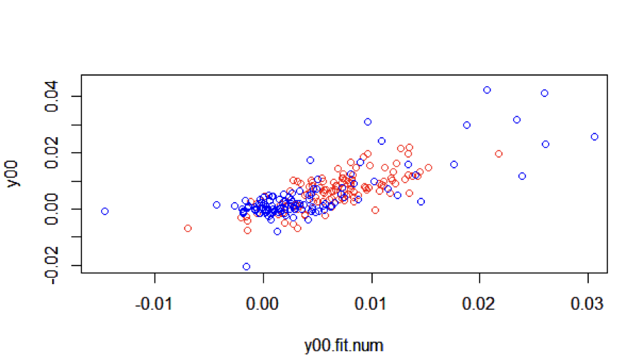
Figure 14: R-square- First 10 years (Red), Last 10 years (Blue)
In figure 14, we have red points representing the first 10 years and blue points representing the last 10 years.
For the last 10 years data, there are many months where the predictions are quite big. There is much greater variability in the last 10 years
4.2 Coefficients Table
For the first 10 years and last 10 years, t-values and p-values are shown in the table below along with statistically significant coefficients in the overall model i.e., p-value < 0.05
4.3 Standard Deviation
For the first 10 years, the Standard Deviation i.e., square root of sigma^2 for logarithmic data is 0.004099652 and for actual data is 1.004206 on the original scale.
For the last 10 years, the Standard Deviation i.e., square root of sigma^2 for logarithmic data is 0.005545686 and for actual data is 1.005561 on the original scale.
The higher standard deviation for the last 10 years data is evident in figures 13 and 14.
5. Forecasting Values
5.1 First 10 Years
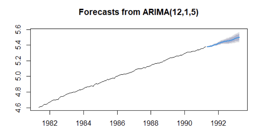
We have taken the data of the first 10 years which fit the best model ARIMA identified by us and predicted the next 24 values i.e., next 2 years data and compared the forecasted values with the original values.
In the below figure, the blue highlighted graph shows the predicted Producer Price Index for the Pharmaceutical Industry.
Using the percentage error formula, We have calculated percentage error for the values. And the mean percentage error is 0.7728233 %
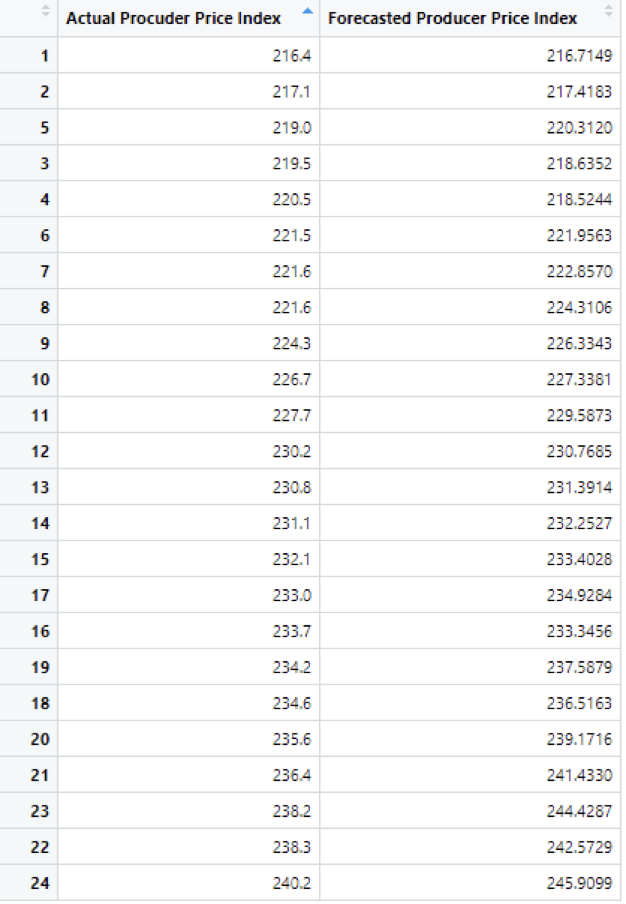
Table 3: Actual vs Forecasted values of the the 11th and 12th years
The above table shows the Actual and Forecasted values of Producer Price Index which are 24 months ahead of our data.
5.2 Last 10 Years
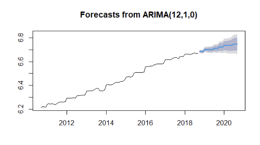
We have taken the data from September 2010 to August 2018 i.e., 8 years and fit the best model ARIMA identified by us and predicted the next 24 values i.e., till August 2020 and then compared the forecasted values with the original values.
In the below figure, the blue highlighted graph shows the predicted logarithmic data of Producer Price Index for the Pharmaceutical Industry.
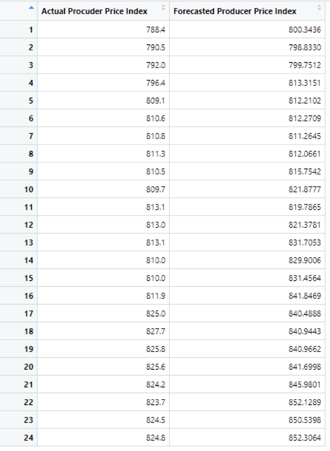
The below table shows the Actual and Forecasted values. Using the percentage error formula, We have calculated percentage error for the values. And the mean percentage error is 1.723034%
Conclusion and Future Scope
The pharmaceutical industry has never before been called upon to solve rapid response issues on a global scale. Although during World War II the production of penicillin was truly an unprecedented engineering feat, it cannot be compared with meeting worldwide pandemic vaccine requirements. Right now is the time for novel solutions.
Meeting the needs of the global community for vaccine during a pandemic outbreak will require exponential improvements in today’s capabilities. It is likely that such advances will have to be made across many fronts to meet the time and volume requirements.
Predicting the Producer Price Index for the upcoming months is necessary for the times when the vaccine needs to be produced in large scale to estimate and to be prepared.
For future scope, the methodology can be extended to have an adaptive time series forecast of the index.
Further research would be focused on building the most effective adaptive models for forecasting and future work could address extending the methodology to build adaptive time series models and such extension would present interesting challenges. The adaptive model is important to allow for regime changes in the process and so the extension to adaptive models would be sensitive to the potential for changes over time but accommodate at the larger time periods if the data is consistent with stable regime over the analysis period.
References
- https://fred.stlouisfed.org/series/PCU325412325412
- https://www.bls.gov/ppi/
- https://www.ftc.gov/sites/default/files/documents/cases/2000/03/genevaabbpttanalysis.htm
- https://haz-map.com/Industries/119
- https://www.abpi.org.uk/medicine-discovery/covid-19/what-are-pharmaceutical-companies-doing-to-tackle-the-disease/
- nae.edu/7640/PharmaceuticalPreparednessforaPandemic
- https://www.rdocumentation.org/packages/forecast/versions/8.13/topics/ndiffs
Appendix I
Ndiffs:
Number Of Differences Required For A Stationary Series.
Function to estimate the number of differences required to make a given time series stationary. Ndiffs estimates the number of first differences necessary.
Acknowledgements
The satisfaction in the execution of this work would be incomplete without expressing my sincere gratitude to all those people whose constant guidance and encouragement made it possible.
Foremost, I would like to express my deep sense of gratitude and august regards to my professor Dr. Peter Kempthorne, Department of Mathematics on financial mathematics and statistics, Massachusetts Institute of Technology, for his unflinching motivation and supervision throughout the coursework and project completion. His untiring efforts in completing the course has helped me understand the concepts and utilize them in our project.
About the author

Roshna Chaik
Roshna graduated from Osmania university in 2019. She is currently Working at J.P Morgan Chase as a Software Engineer.